 | Making a Biome Prediction Artificial Neural Network2022 February 11th |
GitHub Repo: DrPlantabyte / Biome-Prediction-ML
In this project, my aim is to use Python machine learning libraries to create an articficial neural network model for predicting biome classification based on a limited set of environmental parameters, using freely available satellite data to train the model.
What is a biome?
Functionally speaking, a biome is the habitat created by the plants and geology in a given region. Forest, grassland, desert, and deep ocean are all examples of a biome. While there are many different ways of defining biomes, for this project I will be the International Geosphere-Biosphere Programme (IGBP) land cover classification system, which has 17 biome classifications:
- Evergreen needleleaf forest
- Evergreen broadleaf forest
- Deciduous needleleaf forest
- Deciduous broadleaf forest
- Mixed forest
- Closed shrubland
- Open shrubland
- Woody savanna
- Savanna
- Grassland
- Permanent wetland
- Cropland
- Urban and built-up landscape
- Cropland/natural vegetation mosaics
- Snow and ice
- Barren
- Water bodies
What is an artificial neural network?
Similar to biological brains, artificial neural networks are made of interconnected pieces, called nodes, which each perform a small calculation that is then passed on to another node. By playing with the connections between the nodes, the machine learning algorithm is able to evolve the web of nodes from a useless heap into a decision tree that outputs a prediction in it's output node based on the states of the input nodes.
One should not get too carried away by the comparison of artificial neural networks and biological brains. While the high-level principle is the same, biological neurons perform different kinds of calculations than machine learning nodes, and a typical animal brain has millions to trillions of neurons while most machine learning neural network are limited to a few thousand nodes.
What will be the inputs and outputs?
The existing land cover maps already provide biome classification for any location on Earth. However, this is not very useful for hypotheticals, such as what will the landscape look like after another century of global warming? Or what might it have looked like in the past? Or what should the biome maps of Westeros or Middle Earth look like?
Therefore my prediction model will only use easily predictable inputs: average yearly min and max temperature and total annual rainfall amount and standard deviation (to capture seasonality of rainfall). The input data will come from freely available satellite remote sensing data products.
The game plan
My strategy for building this biome prediction model is as follows:
- Download land cover classification, temperature, and rainfall data from NASA
- Clean the data to put everything on the same scale and omit locations with missing data
- Train a classification artificial neural network, using 80% of data pixels for training and 20% for validation, then use the trained model to make a graph of biome classification as a function of min/max temp & rainfall
Step 0: Setup
First thing I do is grab my handy-dandy Python virtual environment bash script:
#!/bin/bashif [ "$#" -ne 2 ]; thenecho "Wrong arguments. Usage:"echo "$0 venv_name requirements_file"exit 1fiVENV_NAME="$1"REQ_FILE="$2"if test ! -d "$VENV_NAME"; thenpython3 -m venv "$VENV_NAME"echo "*" > "$VENV_NAME"/.gitignoresource "$VENV_NAME"/bin/activatepip install --upgrade pippip install -r "$REQ_FILE"pip freeze > "$VENV_NAME"/requirements.txtdeactivatefi
And then I run it to make a python virtual environment with the following requirements.txt file:
numpyrequestsnetCDF4h5pymodis-toolsscipyscikit-learnwxPythonmatplotlibpandaskerastensorflowpygdal
Note that the python package for GDAL is very difficult and frustrating to install. I will not be detailing how to install GDAL here (it involves installing/compiling GDAL to your system first, then installing the matching version of pygdal from pip). If you're ever required to get GDAL with python bindings up and running in a virtual environment, you have my sympathies.
After installation is complete, I create a PyCharm project and get to work on step 1: downloading the data.
Step 1: Downloading the data
While satellite data is available for download from various NASA websites, manually downloading all the files will be quite tedious. For this reason, I will be using the requests library to download the files by HTTP GET protocol.
The first product to download is the MODIS Terra+Aqua Combined Land Cover product, which can be downloaded from the associate USGS site. For simplicity's sake, I'm using the 0.05 degree Climate Modeling Grid (CMG) resolution data, which is stored in simple Mercator projection (aka "longitude/latitude") geometry. For serious work, I'd go for the finer resolutions, which are stored as tiled pieces of a sinusoidal projection (detailed description here).
Browsing through the site, I find that the data is stored in HDF format, at a URL with the following structure: https://e4ftl01.cr.usgs.gov/MOTA/MCD12C1.006/(YEAR).01.01/MCD12C1.A2001001.006.(SOME NUMBERS).hdf, where (YEAR) is the year of interest and (SOME NUMBERS) is a long string of numbers that is slightly different for each file. It's easy enough to scrape the full filename from the website:
import requests, redef get_landcover_URL_for_year(year):html = requests.get('https://e4ftl01.cr.usgs.gov/MOTA/MCD12C1.006/%s.01.01/' % year).content.decode('UTF-8')filename = re.findall('MCD12C1.*?\\.hdf', html)[0]return 'https://e4ftl01.cr.usgs.gov/MOTA/MCD12C1.006/%s.01.01/%s' % (year, filename)
However, a NASA Earthdata account is required to access the data, so if I try this:
import os, sys, re, requestsfrom os import pathdef download_landcover_for_year(year):download_URL = get_landcover_URL_for_year(year)local_filename = path.join('data', 'landcover-%s.hdf' % year)print('Downloading %s to %s...' % (download_URL, local_filename))with requests.get(download_URL, stream=True) as r:r.raise_for_status()with open(local_filename, 'wb') as f:for chunk in r.iter_content(chunk_size=2**20):f.write(chunk)print('...Download complete!')download_landcover_for_year(2002)
I won't get the file to download. Instead, I'll get the requests.exceptions.HTTPError: 401 Client Error: Unauthorized for url error message. Fortunately, there's a new modis-tools Python library available via pip which handles the messy business of scraping MODIS data for us.
import os, sys, re, requestsfrom os import pathfrom modis_tools.auth import ModisSessionfrom modis_tools.resources import CollectionApi, GranuleApifrom modis_tools.granule_handler import GranuleHandlerdef download_MODIS_product(short_name, version, start_date, end_date, dest_dirpath, username, password):os.makedirs(dest_dirpath, exist_ok=True)modis_session = ModisSession(username=username, password=password)# Query the MODIS catalog for collectionscollection_client = CollectionApi(session=modis_session)collections = collection_client.query(short_name=short_name, version=version)granule_client = GranuleApi.from_collection(collections[0], session=modis_session)granules = granule_client.query(start_date=start_date, end_date=end_date)print('Downloading %s to %s...' % (short_name, dest_dirpath))GranuleHandler.download_from_granules(granules, modis_session, path='data')print('...Download complete!')os.makedirs('data', exist_ok=True)username = input('Earth Data Username: ')password = input('Earth Data Password: ')product = 'MCD12C1'version = '006'start_date = '2017-01-01'end_date = '2017-12-31'dest_dirpath = 'data'download_MODIS_product(product, version, start_date, end_date, dest_dirpath, username, password)
Now for the other satellite products for temperature and rainfall. I head back to the MODIS website to find the land surface temperature (LST) product MOD21C3 and then peek at it in the Earth Data browser to make sure it's what I want (it is). Unfortunately, there is no precipitation product for MODIS. Instead, I need to get my data from GPM. The GPM_3IMERGM product (monthly rainfall) looks good, but it needs to be downloaded by URL (there's no equivalent of the modis-tools package).
After a bit of frustration, I finally figured out that there is a URL redirect during authentication, thus to download a GPM file by URL:
import os, sys, re, requestsfrom os import pathdef download_GPM_L3_product(short_name, version, year, month, dest_dirpath, username, password):http_session = requests.session()if(month < 10):month_str = '0'+str(month)else:month_str = str(month)src_url = 'https://gpm1.gesdisc.eosdis.nasa.gov/data/GPM_L3/%s.%s/%s/3B-MO.MS.MRG.3IMERG.%s%s01-S000000-E235959.%s.V06B.HDF5' % (short_name, version, year, year, month_str, month_str)http_session.auth = (username, password)# note: URL gets redirectedredirect = http_session.request('get', src_url)filename = src_url.split('/')[-1]dest_filepath = path.join(dest_dirpath, filename)# NOTE the stream=True parameter belowprint('Downloading %s to %s...' % (redirect.url, dest_filepath))with http_session.get(redirect.url, auth=(username, password), stream=True) as r:r.raise_for_status()with open(dest_filepath,'wb') as f:for chunk in r.iter_content(chunk_size=1048576):f.write(chunk)print('...Download complete!')data_dir = 'data'username = input('Earth Data Username: ')password = input('Earth Data Password: ')year = 2017for month in range(1, 13):download_GPM_L3_product('GPM_3IMERGM', '06', year, month, data_dir, username, password)
Hooray! Data downloads! Note that for the GPM downloads to work, you must first add NASA GESDISC DATA ARCHIVE to your list of approved applications in Earth Data, otherwise the files will contain html instead of satellite data.
Finally, I decide to limit my data to 3 years from the start of 2015 to the end of 2017, so as not to completely fill my hard drive.
def main():print("Starting %s..." % sys.argv[0])# find and download datadata_dir = 'data'username = input('Earth Data Username: ')password = input('Earth Data Password: ')for year in range(2015, 2018):for month in range(1, 13):download_GPM_L3_product('GPM_3IMERGM', '06', year, month, data_dir, username, password)download_MODIS_product('MOD21C3', '061', '%s-01-01' % year, '%s-12-31' % year, data_dir, username, password)download_MODIS_product('MCD12C1', '006', '%s-01-01' % year, '%s-12-31' % year, data_dir, username, password)#print("...Done!")
Step 2: Data cleaning
Now it's time to take the data, discard anything that is poor quality or unnecesary, and then reformat it in a way that is more friendly to machine learning. As a brief reminder, my model inputs and outputs are:
Inputs
- Average yearly temperature minimum
- Average yearly temperature maximum
- Average annual rainfall
- Standard deviation of monthly rainfall totals
Outputs
- Predicted IGBP classification
So the goal therefore is to calculate those values for all (or a subset) of the satellite data and save it in a table format (eg DataFrame)
The first step is, of course, to open the hdf files to access the data in the first place. I start by installing HDF View to take a look at the files with a GUI, as this is a much faster way of exploring the data structure. Then using the h5py module, I'm able to see the rainfall data file structure with the following Python code:
import os, sys, h5pyfrom os import pathdef print_structure(hdf: h5py.File):for key in hdf.keys():_print_structure(hdf.get(key), 0)def _print_structure(node, indent):# recursive implementationprint('\t'*indent, end='')print(node.name)if type(node) == h5py._hl.group.Group:for key in node.keys():_print_structure(node.get(key), indent + 1)elif type(node) == h5py._hl.dataset.Dataset:print('\t' * (indent+1), end='')print('Dataset: dtype = %s; shape = %s; compression = %s; total bytes = %s' % (node.dtype, node.shape, node.compression, node.nbytes))else:# unknown typeprint('\t' * (indent+1), end='')print(type(node))data_dir = path.join('data')hdf_file = path.join(data_dir, '3B-MO.MS.MRG.3IMERG.20160801-S000000-E235959.08.V06B.HDF5')with h5py.File(hdf_file, 'r') as hdf:print_structure(hdf)
Then I'm able to look at the rainfall data with the following code:
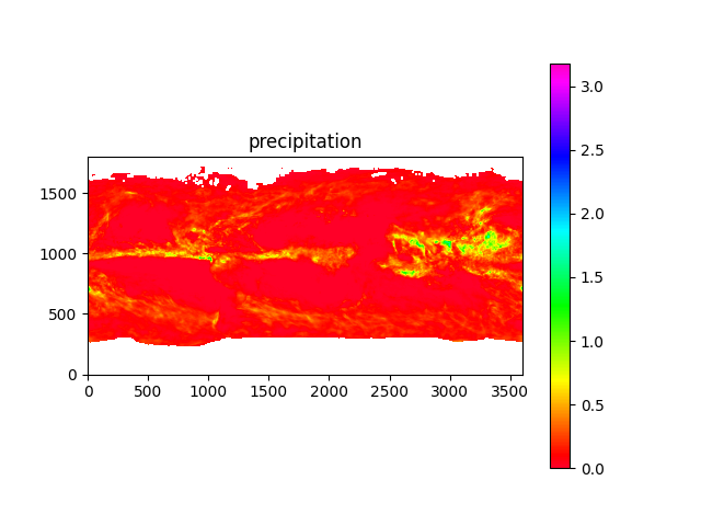
import os, sys, h5py, numpyfrom os import pathfrom matplotlib import pyplotdata_dir = path.join('data')hdf_file = path.join(data_dir, '3B-MO.MS.MRG.3IMERG.20160801-S000000-E235959.08.V06B.HDF5')# note: precipitation data has units of mm/hr, and is the month-long average of per-hour rateswith h5py.File(hdf_file, 'r') as hdf:print_structure(hdf)for data_type in ['precipitation', 'randomError', 'gaugeRelativeWeighting', 'probabilityLiquidPrecipitation', 'precipitationQualityIndex']:data_map = hdf.get('/Grid/%s' % data_type)[0].T# note: -9999.9 means "no data"print(data_type, data_map.min(),'-',data_map.max())pyplot.clf()pyplot.imshow(data_map.clip(0,numpy.inf), origin='lower', cmap='gist_rainbow')pyplot.colorbar()pyplot.title(data_type)pyplot.savefig('precip_map_%s.png' % data_type)pyplot.show()
However, the MODIS data is in HDF4 format, which is not supported by h5py. I have to use the GDAL library instead:
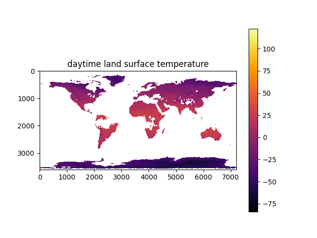
import os, sys, h5py, numpy, jsonfrom os import pathfrom matplotlib import pyplotfrom osgeo import gdaldef print_modis_structure(dataset: gdal.Dataset):metadata_dict = dict(dataset.GetMetadata_Dict())metadata_dict['Subsets'] = dataset.GetSubDatasets()print(dataset.GetDescription(), json.dumps(metadata_dict, indent=" "))data_dir = path.join('data')modis_file = path.join(data_dir, 'MOD21C3.A2015001.061.2021320021656.hdf')modis_dataset: gdal.Dataset = gdal.Open(modis_file)print_modis_structure(modis_dataset)scale_factor = 0.02data_name = 'Daytime LST'data_map = gdal.Open(modis_dataset.GetSubDatasets()[5][0]).ReadAsArray()print(data_map.shape)print(data_name, data_map.min(), '-', data_map.max())pyplot.clf()kelvin = data_map.astype(numpy.float32) * scale_factorkelvin[kelvin == 0] = numpy.nanpyplot.imshow(kelvin - 273.15, origin='upper', cmap='inferno')pyplot.colorbar()pyplot.title(data_name)pyplot.savefig('temperature_map_%s.png' % data_name)pyplot.show()
With a little bit of clean-up, my ode now looks like this:
import os, sys, h5py, numpy, jsonfrom os import pathfrom matplotlib import pyplotfrom osgeo import gdaldef plot_data_map(data_map: numpy.ndarray, title: str, origin='lower', cmap='gist_rainbow'):pyplot.clf()pyplot.imshow(data_map, origin=origin, cmap=cmap)pyplot.colorbar()pyplot.title(title)pyplot.savefig('%s.png' % title)pyplot.show()def get_modis_data(modis_root_dataset: gdal.Dataset, subset_index):data_map = gdal.Open(modis_root_dataset.GetSubDatasets()[subset_index][0]).ReadAsArray()return data_mapdef print_modis_structure(dataset: gdal.Dataset):metadata_dict = dict(dataset.GetMetadata_Dict())metadata_dict['Subsets'] = dataset.GetSubDatasets()print(dataset.GetDescription(), json.dumps(metadata_dict, indent=" "))def print_structure(hdf: h5py.File):for key in hdf.keys():_print_structure(hdf.get(key), 0)def _print_structure(node, indent):# recursive implementationprint('\t'*indent, end='')print(node.name)if type(node) == h5py._hl.group.Group:for key in node.keys():_print_structure(node.get(key), indent + 1)elif type(node) == h5py._hl.dataset.Dataset:print('\t' * (indent+1), end='')print('Dataset: dtype = %s; shape = %s; compression = %s; total bytes = %s' % (node.dtype, node.shape, node.compression, node.nbytes))else:# unknown typeprint('\t' * (indent+1), end='')print(type(node))data_dir = path.join('data')biome_map_file = path.join(data_dir, 'MCD12C1.A2015001.006.2018053185652.hdf')biome_map_ds = gdal.Open(biome_map_file)print_modis_structure(biome_map_ds)biome_map = get_modis_data(biome_map_ds, 0)plot_data_map(biome_map, 'IGBP cover type', origin='upper', cmap='gist_rainbow')biome_map_ds = None # GDAL implements .Close() on object de-referencedel biome_map_filedel biome_mapdel biome_map_dssample_LST_file = path.join(data_dir, 'MOD21C3.A2016061.061.2021346202936.hdf')LST_ds = gdal.Open(sample_LST_file)print_modis_structure(LST_ds)LST_map = get_modis_data(LST_ds, 5).astype(numpy.float32) * 0.02LST_map[LST_map <= 0] = numpy.nanplot_data_map(LST_map-273.15, 'daytime land surface temperature', origin='upper', cmap='inferno')LST_ds = None # GDAL implements .Close() on object de-referencedel sample_LST_filedel LST_mapdel LST_dssample_rainfall_file = path.join(data_dir, '3B-MO.MS.MRG.3IMERG.20160801-S000000-E235959.08.V06B.HDF5')# note: precipitation data has units of mm/hr, and is the month-long average of per-hour rateswith h5py.File(sample_rainfall_file, 'r') as hdf:print_structure(hdf)data_type = 'precipitation'data_map = hdf.get('/Grid/%s' % data_type)[0].T# note: -9999.9 means "no data"print(data_type, data_map.min(),'-',data_map.max())masked_data = data_map.astype(numpy.float32)masked_data[masked_data < 0] = numpy.nanplot_data_map(masked_data * (24*30), '30-day Precipitation', origin='lower', cmap='gist_rainbow')
Note that to close a GDAL data file, you set the data set variable to None. This is not a common resource management pattern in Python, but it's best not to fight the GDAL library.
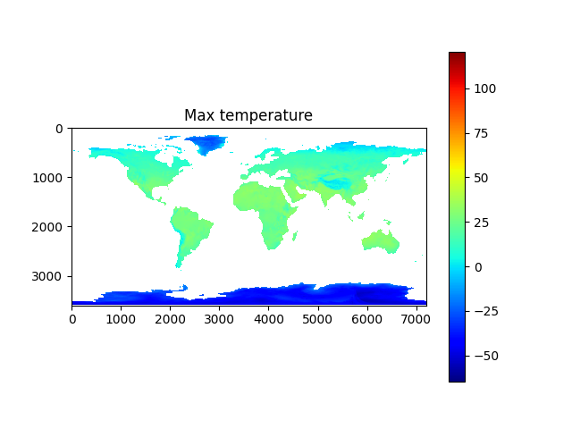
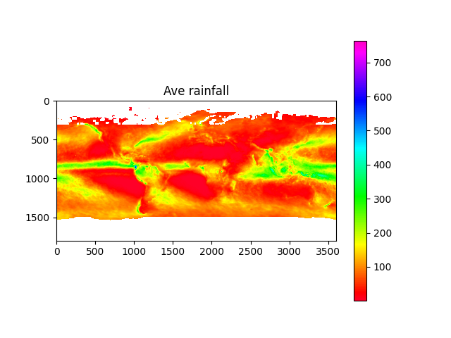
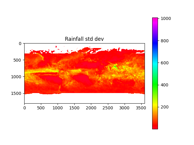
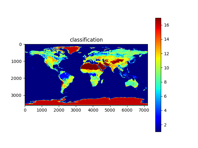
Here's what the data looks like:
Now remembering the model inputs listed above, the data I actually have is:
- Monthly average rate of precipitation in mm/hr
- Monthly average day and night time land surface temperature in degrees Kelvin
- IGBP classification
Thus I'll have to process the data to produce the actual inputs I want to use for training the machine learning model.
But first, since satellite data processing is rather time consuming, I add a file cache using Python's pickle package to save the data after I process it so that subsequent runs take much less time:
import pickledef load_pickle(filepath):if path.exists(filepath):with open(filepath, 'rb') as fin:return pickle.load(fin)else:return Nonedef save_pickle(filepath, data):with open(filepath, 'wb') as fout:pickle.dump(data, fout)
With that out of the way, it's time to plug-and-chug!
import os, sys, h5py, numpy, json, math, picklefrom os import pathfrom matplotlib import pyplotfrom osgeo import gdaldata_dir = path.join('data')# calculate minand max temperaturesmin_temp_map = load_pickle(path.join(data_dir, 'min_temp_map.pickle'))max_temp_map = load_pickle(path.join(data_dir, 'max_temp_map.pickle'))if min_temp_map is None or max_temp_map is None:min_temp_map = numpy.zeros((3600,7200), dtype=numpy.float32)max_temp_map = numpy.zeros_like(min_temp_map)lst_files = [x for x in os.listdir(data_dir) if x.startswith('MOD21C3')]lst_date_dict = {}for f in lst_files:ds: gdal.Dataset = gdal.Open(path.join(data_dir, f))ddate = ds.GetMetadata_Dict()["RANGEBEGINNINGDATE"]yearmo = ddate[0:4]+ddate[5:7]print(yearmo)lst_date_dict[yearmo] = fddate = Noneds = Nonecount = 0for year in range(2015, 2018):print('processing year %s temperature...' % year)count += 1annual_max_temp_map = Noneannual_min_temp_map = Nonefor month in range(1, 13):print('\tMonth %s...' % month)yearmo = str(year) + to2digit(month)lst_filename = lst_date_dict[yearmo]ds: gdal.Dataset = gdal.Open(path.join(data_dir, lst_filename))daytime_lst = get_modis_data(ds, 5).astype(numpy.float32) * 0.02daytime_lst[daytime_lst < 150] = numpy.nan # remove bad valuesnighttime_lst = get_modis_data(ds, 6).astype(numpy.float32) * 0.02nighttime_lst[nighttime_lst < 150] = numpy.nanif annual_max_temp_map is None:annual_max_temp_map = daytime_lstif annual_min_temp_map is None:annual_min_temp_map = nighttime_lstannual_max_temp_map = numpy.nanmax((annual_max_temp_map, daytime_lst, nighttime_lst), axis=0)annual_min_temp_map = numpy.nanmin((annual_min_temp_map, daytime_lst, nighttime_lst), axis=0)del daytime_lstdel nighttime_lstds = Nonedel dsmin_temp_map = min_temp_map + annual_min_temp_mapmax_temp_map = max_temp_map + annual_max_temp_mapmin_temp_map = min_temp_map / countmax_temp_map = max_temp_map / countsave_pickle(path.join(data_dir, 'min_temp_map.pickle'), min_temp_map)save_pickle(path.join(data_dir, 'max_temp_map.pickle'), max_temp_map)plot_data_map(min_temp_map-273.15, 'Min temperature', origin='upper', cmap='jet')plot_data_map(max_temp_map-273.15, 'Max temperature', origin='upper', cmap='jet')# calculate average and std dev of rainfallave_precip_map = load_pickle(path.join(data_dir, 'ave_precip_map.pickle'))stdev_precip_map = load_pickle(path.join(data_dir, 'stdev_precip_map.pickle'))if ave_precip_map is None or stdev_precip_map is None:precip_time_series = Nonefor year in range(2015, 2018):print('processing year %s rainfall...' % year)for month in range(1, 13):print('\tMonth %s...' % month)precip_filename = '3B-MO.MS.MRG.3IMERG.%s%s01-S000000-E235959.%s.V06B.HDF5' % (year, to2digit(month), to2digit(month))with h5py.File(path.join(data_dir, precip_filename), 'r') as hdf:## correct to same orientation as modis dataprecip_map = numpy.flip(hdf.get('/Grid/precipitation')[0].T, axis=0).astype(numpy.float32)#precip_map = numpy.flip(hdf.get('/Grid/gaugeRelativeWeighting')[0].T, axis=0).astype(numpy.float32)precip_map[precip_map < 0] = numpy.nanprecip_map = precip_map * (24 * 365.24/12) # convert to monthly totalif precip_time_series is None:precip_time_series = precip_mapelif len(precip_time_series.shape) == 2:#precip_time_series = numpy.stack((precip_time_series, precip_map), axis=0)else:precip_time_series = numpy.concatenate((precip_time_series, [precip_map]))ave_precip_map = numpy.mean(precip_time_series, axis=0)stdev_precip_map = numpy.std(precip_time_series, axis=0)save_pickle(path.join(data_dir, 'ave_precip_map.pickle'), ave_precip_map)save_pickle(path.join(data_dir, 'stdev_precip_map.pickle'), stdev_precip_map)plot_data_map(ave_precip_map, 'Ave rainfall', origin='upper')plot_data_map(stdev_precip_map, 'Rainfall std dev', origin='upper')# retrieve biomes from 2017biome_map_file = path.join(data_dir, 'MCD12C1.A2017001.006.2019192025407.hdf')biome_map_ds = gdal.Open(biome_map_file)biome_map = numpy.copy(get_modis_data(biome_map_ds, 0))+1print('found biome codes: %s' % numpy.unique(biome_map))biome_map_ds = Nonedel biome_map_dsplot_data_map(biome_map, 'classification', origin='upper', cmap='jet')
Ahhh... Yes, I love the smell of good clean data in the morning!
But we're not quite done yet. The above procedure produces maps of the relevant data, but the machine learning algorithms expect tables of data. Furthermore, the input data is in Mercator projection so it is overly biased towards polar data. Thus I'll resample it with sinusoidal projection (and I'll be down-sampling to reduce the volume of data in the interest of time), storing the sampled data as a linearized table instead of an image. Easy enough:
import os, sys, numpy, math, picklefrom pandas import DataFramefrom os import path# sample with sinusoidal projectionmin_temps = numpy.asarray([], dtype=numpy.float32)max_temps = numpy.asarray([], dtype=numpy.float32)ave_rain = numpy.asarray([], dtype=numpy.float32)dev_rain = numpy.asarray([], dtype=numpy.float32)biomes = numpy.asarray([], dtype=numpy.uint8)deg2rad = math.pi/180rad2deg = 180/math.pispatial_resolution_degrees = 0.1for lat in numpy.linspace(-90,90-spatial_resolution_degrees,int(180/spatial_resolution_degrees)):# note: Y = 0 is north pole, positive latitude is northern hemisphere# note: rain map is 0.1 degree pixels, others are 0.05 degree pixelslongitudes = numpy.linspace(-180, 180-spatial_resolution_degrees, int(rad2deg*numpy.cos(lat*deg2rad)))if len(longitudes) == 0: # don't sample the polescontinue#print('latitude %s (%s longitudes sampled)' % (lat, len(longitudes)))biome_row = int((90 - lat) * 20)lst_row = int((90 - lat) * 20)precip_row = int((90 - lat) * 10)biome_cols = ((longitudes + 180) * 20).astype(dtype=numpy.int32)lst_cols = ((longitudes + 180) * 20).astype(dtype=numpy.int32)precip_cols = ((longitudes + 180) * 10).astype(dtype=numpy.int32)min_temps = numpy.concatenate((min_temps, min_temp_map[lst_row].take(lst_cols)))max_temps = numpy.concatenate((max_temps, max_temp_map[lst_row].take(lst_cols)))ave_rain = numpy.concatenate((ave_rain, ave_precip_map[precip_row].take(precip_cols)))dev_rain = numpy.concatenate((dev_rain, stdev_precip_map[precip_row].take(precip_cols)))biomes = numpy.concatenate((biomes, biome_map[biome_row].take(biome_cols)))data_table: DataFrame = DataFrame.from_dict({"Temperature Min (C)": min_temps-273.15,"Temperature Max (C)": max_temps-273.15,"Annual Rainfall (mm/yr)": ave_rain*12,"Monthly Rainfall Std. Dev. (% mean)": (dev_rain/ave_rain) * 100,"Classification (IGBP code)": biomes})## now remove rows with nansdata_table = data_table.dropna()save_pickle(path.join(data_dir, 'data_table.pickle'), data_table)print(data_table)
Excellent! Step 2 is done! Now I can train my model with the data saved in data/data_table.pickle.
Step 3: Train the machine
Alright! Time for the main course!
The first thing to do is to normalize the data to a range of approximately 0 to 1, because machine learning models learn faster with normalized data (for reasons I won't go into here).
I take a peak at the data with the following code:
import os, sys, numpy, picklefrom pandas import DataFramefrom os import pathdata_dir = path.join('data')data_table: DataFrame = load_pickle(path.join(data_dir, 'data_table.pickle'))for col in data_table.columns:col_data = data_table[col]print('%s\t[%s, %s]' % (col, numpy.min(col_data), numpy.max(col_data)))
which prints:
Temperature Min (C) [-45.863327, 28.910004]Temperature Max (C) [-33.58333, 40.070007]Annual Rainfall (mm/yr) [1.2830898, 6305.9707]Monthly Rainfall Std. Dev. (% mean) [19.385046, 420.88327]Classification (IGBP code) [1, 17]
I'm going to use the MinMaxScaler from sklearn.preprocessing. The sklearn proprocessing methods can be a bit fidgety, so always check your work:
import os, sys, numpy, picklefrom pandas import DataFramefrom os import pathfrom sklearn.preprocessing import MinMaxScalernormalizer = MinMaxScaler()x_data = normalizer.fit_transform(data_table.drop('Classification (IGBP code)', axis=1))y_data = numpy.asarray(data_table['Classification (IGBP code)'])scaling_vector_slope = normalizer.data_range_scaling_vector_offset = normalizer.data_min_print('normalizer vectors [slope offset]:\n', numpy.stack((scaling_vector_slope, scaling_vector_offset), axis=1))save_pickle(path.join(model_dir, 'normalizer.pickle'), normalizer)print('x_data.shape == %s\ty_data.shape == %s' % (x_data.shape, y_data.shape))
Next, randomly split the data into training and testing (I'll use an 80%:20% split here):
import numpyrow_count = x_data.shape[0]indices = numpy.indices([row_count])[0]numpy.random.shuffle(indices)x_training = x_data.take(indices[0:int(0.80*row_count)], axis=0)y_training = y_data.take(indices[0:int(0.80*row_count)], axis=0)x_testing = x_data.take(indices[int(0.80*row_count):row_count], axis=0)y_testing = y_data.take(indices[int(0.80*row_count):row_count], axis=0)
Finally, time to build and train the model. I opt for the Keras sequential model with three layers of dense networks, just because this is one of the easier types of machine learning models to work with. If I revisit this to fine-tune the model, I could use a different kin of model, add more layers, add different kinds of layers, and change the parameters. For now, though, let's keep it simple:
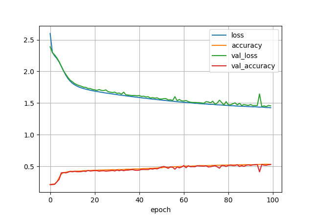
import os, sys, numpy, picklefrom pandas import DataFramefrom os import pathfrom sklearn.preprocessing import MinMaxScalerfrom matplotlib import pyplotimport tensorflow as tffrom tensorflow import kerasmodel = keras.models.Sequential([keras.layers.Dense(300, activation="relu", input_shape=(4,)),keras.layers.Dense(100, activation="relu"),keras.layers.Dense(17+1, activation="softmax") # +1 because Y data is 1-indexed instead of 0-indexed])print('input shape:', model.input_shape)print('output shape:', model.output_shape)model.build()print(model.summary())model.compile(loss=keras.losses.sparse_categorical_crossentropy,optimizer=keras.optimizers.SGD(learning_rate=0.03),metrics=['accuracy'])print('Starting to train...')print('x_training.shape == %s\ty_training.shape == %s' % (x_training.shape, y_training.shape))history = model.fit(x_training, y_training, batch_size=100, epochs=100, validation_split=0.1)print('...training done!')# see the evolution of the modelDataFrame(history.history).plot()pyplot.grid(True)#pyplot.gca().set_ylim(0,1)pyplot.xlabel("epoch")pyplot.show()
Success!
But how good is the model? Enter the test data:
test = model.evaluate(x_testing, y_testing) # returns loss, metrics...print('Accuracy on test data: %.2f%%' % (100*test[1]))
The bottom line: 54.15% percent accurate. That's pretty bad, but not surprising, as I already know that biomes have more important environmental inputs than temperature and rainfall. But I'm not aiming for accurate in this project, it's just for fun. So let's give it a test using the weather of San Diego where I grew up:
igbp_names = ['ERROR', 'Evergreen needleleaf forest', 'Evergreen broadleaf forest', 'Deciduous needleleaf forest','Deciduous broadleaf forest', 'Mixed forest', 'Closed shrubland', 'Open shrubland', 'Woody savanna','Savanna', 'Grassland', 'Permanent wetland', 'Cropland', 'Urban and built-up landscape','Cropland/natural vegetation mosaics', 'Snow and ice', 'Barren', 'Water bodies']print("Test the prediction model:")T_min = float(input("Enter min temperature (C): "))T_max = float(input("Enter max temperature (C): "))rain = float(input("Enter annual rainfall (mm): "))rain_dev = float(input("Enter rainfall std dev (% of average): %"))x = normalizer.transform([numpy.asarray([T_min, T_max, rain, rain_dev])])class_predictions = model.predict([x])[0]print(class_predictions.round(2))predicted_biome = numpy.argmax(class_predictions)print("Predicted IGBP code: %s (%s)" % (predicted_biome, igbp_names[predicted_biome]))>>>> Test the prediction model:>>>> Enter min temperature (C): 5>>>> Enter max temperature (C): 40>>>> Enter annual rainfall (mm): 200>>>> Enter rainfall std dev (% of average): %50[0. 0. 0. 0. 0. 0. 0. 0.01 0.5 0. 0. 0.02 0. 0.040. 0. 0. 0.43]Predicted IGBP code: 8 (Woody savanna)
Woody savanna is actually pretty close to the chaparrel of southern California, so it's a good prediction. To briefly explain how I read the model, the output of the model is an array of probabilities for each IGBP classification. Thus the array index with the highest probability is the predicted classification (selected using numpy.argmax()). Index 0 in this case is unused, since the IGBP codes start at 1, not zero.
To visualize the predictions, I make a number of plots with gradients of temperature and rainfall. The result looks pretty cool:
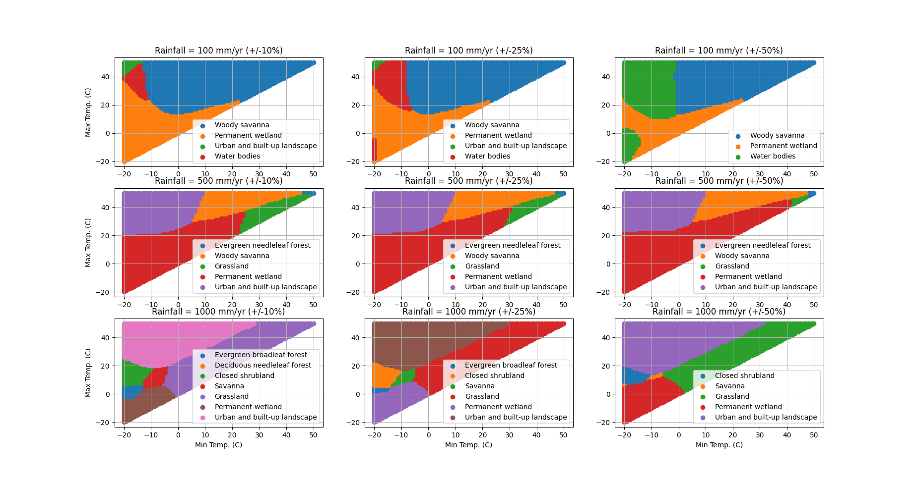
Mission accomplished!
Epilog
I made this project to demonstrate the use of machine learning with satellite data. It took me about a day's worth of work for each step, and I'm only scratching the surface of satellite products and machine learning. You are welcome to use my project as the starting point for your own machine learning adventures, and I hope that my example code and brief explanations help you with the tricky business of data engineering and training. Enjoy!
 Dr. Christopher C. Hall | plantabyte.net